Economics for Engineers
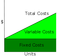
Fixed cost
A fixed cost is a cost that does not change with an increase or decrease in the amount of goods or services produced or sold. Fixed costs are expenses that have to be paid by a company, independent of any business activity.
| Examples | Depreciation, Rent, Salary, Insurance, Tax etc. |
What is a 'Variable Cost'
Examples Material Consumed, Wages, Commission on Sales, Packing Expenses, etc.
Difference Between Fixed Cost and Variable Cost
| BASIS FOR COMPARISON | FIXED COST | VARIABLE COST |
|---|---|---|
| Meaning | The cost which remains same, regardless of the volume produced, is known as fixed cost. | The cost which changes with the change in output is considered as a variable cost. |
| Nature | Time Related | Volume Related |
| Incurred when | Fixed costs are definite, they are incurred whether the units are produced or not. | Variable costs are incurred only when the units are produced. |
| Unit Cost | Fixed cost changes in unit, i.e. as the units produced increases, fixed cost per unit decreases and vice versa, so the fixed cost per unit is inversely proportional to the number of output produced. | Variable cost remains same, per unit. |
| Behavior | It remains constant for a given period of time. | It changes with the change in the output level. |
| Combination of | Fixed Production Overhead, Fixed Administration Overhead and Fixed Selling and Distribution Overhead. | Direct Material, Direct Labor, Direct Expenses, Variable Production Overhead, Variable Selling and Distribution Overhead. |
| Examples | Depreciation, Rent, Salary, Insurance, Tax etc. | Material Consumed, Wages, Commission on Sales, Packing Expenses, etc. |

Marginal cost
In economics, marginal cost is the change in the total cost that arises when the quantity produced is incremented by one unit, that is, it is the cost of producing one more unit of a good.
Cost Estimating and Estimating Models
Engineering economic analysis involves present and future economic factors; thus, it is critical to obtain reliable estimates of future costs, benefits and other economic parameters. Several methods to do so are discussed here.
Estimates can be rough estimates, semi detailed estimates, or detailed estimates, depending on the needs for the estimates.
A characteristic of cost estimates is that errors in estimating are typically nonsymmetric because costs are more likely to be underestimated than overestimated.
Difficulties in developing cost estimates arise from such conditions as one-of-a-kind estimates, resource availability, and estimator expertise. Generally the quality of a cost estimate increases as the resources allocated to developing the estimate increase. The benefits expected from improving a cost estimate should outweigh the cost of devoting additional resources to the estimate improvement.
Several models are available for developing cost (or benefit) estimates.
The per-unit model is a simple but useful model in which a cost estimate is made for a single unit, then the total cost estimate results from multiplying the estimated cost per unit times the number of units.
The segmenting model partitions the total estimation task into segments. Each segment is estimated, then the segment estimates are combined for the total cost estimate.
Cost indexes can be used to account for historical changes in costs. The widely reported Consumer Price Index (CPI) is an example. Cost index data are available from a variety of sources. Suppose A is a time point in the past and B is the current time. Let IVA denote the index value at time A and IVB denote the current index value for the cost estimate of interest. To estimate the current cost based on the cost at time A, use the equation:
Cost at time B = (Cost at time A) (IVB / IVA).
The power-sizing model accounts explicitly for economies of scale. For example, the cost of constructing a six-story building will typically be less than double the construction cost of a comparable three-story building. To estimate the cost of B based on the cost of comparable item A, use the equation
Cost of B = (Cost of A) [ ("Size" of B) / ("Size" of A) ] x
where x is the appropriate power-sizing exponent, available from a variety of sources. An economy of scale is indicated by an exponent less than 1.0 An exponent of 1.0 indicates no economy of scale, and an exponent greater than 1.0 indicates a diseconomy of scale.
"Size" is used here in a general sense to indicate physical size, capacity, or some other appropriate comparison unit.
Learning curve cost estimating is based on the assumption that as a particular task is repeated, the operator systematically becomes quicker at performing the task. In particular, the model is based on the assumption that the time required to complete the task for production unit 2x is a fixed percentage of the time required for production unit x for all positive, integer x. The learning curve slope indicates "how fast" learning occurs. For example, a learning curve rate of 70% represents much faster learning than a rate of 90%. If an operator exhibits learning on a certain task at a rate of 70%, the time required to complete production unit 50, for example, is only 70% of the time required to complete unit 25.
Let b = learning curve exponent
= log (learning curve rate in decimal form) / log 2.0
= log (learning curve rate in decimal form) / log 2.0
Then TN = time estimate for unit N (N = 1, 2, ...)
= (T1) (N)b
= (T1) (N)b
where T1 is the time required for unit 1.
As an example: A learning curve rate is 70%, the operator’s time for the firstt unit is 65 seconds. What is the operator’s time for the 50th unit?
T100 = T1 * (50) ^ b = 65 * (50) ^ -0.5145 = 8.68 min
cost index
A cost index is the ratio of the actual price in a time period compared to that in a selected base period (a defined point in time or the average price in a certain year), multiplied by 100.
How does this PVIFA calculator work?
This financial tool can help when trying to determine the present value interest factor of annuity which is a value that can be used to calculate the present value of an annuity series.
The algorithm behind this PVIFA calculator uses the formula explained here and it requires the interest rate and the number of periods to be given:

Where:
-N = (-1) * Number of periods
r = Assumed interest rate per period
PVIFA definition
In finance theory, PVIFA is the acronym for present value interest factor of annuity which represents a factor that can be used to determine the present value of a series of annuity, the monthly payment needed to payoff a loan or to calculate the PV of an ordinary annuity.
simple interest formula: A = P(1 + rt) where P is the Principal amount of money to be invested at an Interest Rate R% per period for t Number of Time Periods.
Net present value (NPV) is the present value of an investment's expected cash inflows minus the costs of acquiring the investment.
The formula for NPV is: NPV = (Cash inflows from investment) – (cash outflows or costs of investment)
What is the 'Present Value Interest Factor - PVIF'
The present value interest factor (PVIF) is a factor that is utilized to provide a simple calculation for determining the present value dollar amount of a sum of money to be received at some future point in time. For determination or consideration of a series of possible present values, PVIFs are often represented in the form of a table used for calculating the present value of a future sum with varying interest rate and time period combinations. The present value interest factor is based on the foundational financial concept of the time value of money, which states that the present value of a sum of money not to be received until sometime in the future must be discounted from the future amount according to a rate of return that could be earned on capital at the present time.
BREAKING DOWN 'Present Value Interest Factor - PVIF'
The formula for calculating the present value interest factor is as follows:
PVIF = a / (1 + r) ^ n
The "a" represents the future sum to be received, "r" represents the discount interest rate, and "n" represents the number of years or other time period.
Equivalent Annual Annuity
Equivalent Annual Annuity Calculator

Present Worth Analysis
Break- even analysis - BE analysis is also called break even point BEP is the level of production or sales where total sales equal to total cost i.e at break even point there is no loss or profit.
The main objective of break-even analysis is to find the cut-off production volume from where a firm will make profit.

BEP(in units)=fixed cost/contribution per unit
contribution per unit= (selling price per unit - variable cost per unit)
BEP or Break even sales(in rupees)= Fixed cost/profit volume ratio
profit volume ratio =(total contribution /total sales )*100
Or
p/v ratio = (contribution per unit /selling price per unit)*100
Sensitivity Analysis
sensitivity analysis is also called "what if" analysis, analysis and explores what would happen to the viability of the project when some variable likes sales or investment deviates from its expected value.sensitivity analysis varies only one variable at a time e.g to study the effect of an adverse variation in sales, the values of the other underlying variable are maintained at their expected values.
Merit of sensitivity analysis
1.It is very popular method of assessing risk because it shows how robust or vulnerable a project is to changes in values of underlying variables.
2.It indicates whether further work is necessary because if net profit value is highly sensitive to changes in some factor,it may be worthwhile to explore how the vulnerability of the critical factor may be reduced.
3.It is intuitively very appealing because if articulates the concerns the project evaluators normally have.
Demerit of sensitivity analysis
1.It does not provide any idea of the profitability of the change in the variable -only shows what happens to net profit value if there is a change in that variable.
2.In the real world many variables change together whereas in sensitivity analysis only one variable is change at a time.
3.The result of sensitivity analysis may be interpreted by different decision-makers differently -one may accept the project and other may reject the project.
Future worth Analysis


Explain P/V ratio and Contribution.
P/V Ratio:
P/V Ratio (Profit Volume Ratio) is the ratio of contribution to sales which indicates the contribution earned with respect to one rupee of sales. It also measures the rate of change of profit due to change in volume of sales. Its fundamental property is that if per unit sales price and variable cost are constant then P/V Ratio will be constant at all the levels of activities. A change is fixed cost does not affect P/V Ratio. It is calculated as under:
(Contribution * 100) / Sales
(Change in profits * 100) / (Change in sales)
A high P/V Ratio indicates that a slight increase in sales without increase in fixed costs will result in higher profits. A low P/V ratio which indicates low profitability can be improved by increasing selling price, reducing marginal costs or selling products having high P/V ratio.
Contribution:
It is the difference between sales revenue and variable cost (also known as variable cost). Variable cost is the important cost in deciding profitability as fixed costs are ignored by marginal costing.
It can be expressed in two ways:
• Sales Revenue – Variable Cost
• Fixed Cost + Profit
The situation generating higher contribution is treated as a profitable situation.
Explain Break Even Point. How does BEP help in making business decision?
Break Even Point (BEP) is a volume of sales where there is neither loss nor profit. That means contribution is enough to cover the fixed costs.
Thus, we can say that Contribution = Fixed Cost
Any contribution generated after BEP will directly result into profits as the fixed costs are fully covered now. BEP can be computed in two ways:
In terms of Quantity-
Fixed Costs / Contribution per unit
In terms of Amount-
(Fixed Costs) / (P/V Ratio)
BEP (Break Even Point) is the situation where there is neither loss nor profit. At this stage, the contribution is enough to cover the fixed costs i.e contribution is equal to fixed cost. Contribution generated after the break even point will result in profits for the organisation. Profit maximization is the motive of every organisation. Thus, every organisation use BEP as a base to take various decisions in regard to its sales volume and tries to increase it so that total fixed costs can be covered as early as possible and more profits can be earned.
Explain Margin of Safety.
Margin of Safety is the amount of sales which generates profit. In other words, sales beyond Break Even Point are known as Margin of Safety. It is calculated as the difference between total sales and the break even sales. It can be expressed in monetary terms or number of units. It can be expressed as below:
Margin of Safety = Sales – Break Even Sales
= Sales - {(Fixed Cost) / (P/V Ratio)}
= ((Sales * (P/V) Ratio) - Fixed Cost) / (P/V) Ratio
= (Contribution - Fixed Cost) / (P/V) Ratio
= Profit / (P/V) Ratio
The size of margin of safety is an extremely important guide to the financial strength of a business. If margin of safety is large, which indicates that BEP is much below the actual sales, that means business is in a sound condition and reduction in sales will not affect the profit of the business. On the other hand, if margin of safety is low, any loss of sales may be a serious matter. Thus, efforts need to be made to reduce fixed costs, variable costs or increasing the selling price or sales volume to improve contribution and overall P/V Ratio.
What is 'Net Present Value - NPV'
Net Present Value (NPV) is the difference between the present value of cash inflows and the present value of cash outflows. NPV is used in capital budgeting to analyze the profitability of a projected investment or project.
The following is the formula for calculating NPV:
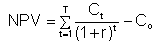
where
Ct = net cash inflow during the period t
Co = total initial investment costs
r = discount rate, and
t = number of time periods
A positive net present value indicates that the projected earnings generated by a project or investment exceeds the anticipated costs. Generally, an investment with a positive NPV will be a profitable one and one with a negative NPV will result in a net loss. This concept is the basis for the Net Present Value Rule, which dictates that the only investments that should be made are those with positive NPV values.
Drawbacks and Alternatives
One primary issue with gauging an investment’s profitability with NPV is that NPV relies heavily upon multiple assumptions and estimates, so there can be substantial room for error. Estimated factors include investment costs, discount rate and projected returns. A project may often require unforeseen expenditures to get off the ground or may require additional expenditure at the project’s end.
Additionally, discount rates and cash inflow estimates may not inherently account for risk associated with the project and may assume the maximum possible cash inflows over an investment period. This may occur as a means of artificially increasing investor confidence. As such, these factors may need to be adjusted to account for unexpected costs or losses or for overly optimistic cash inflow projections.
Payback period is one popular metric that is frequently used as an alternative to net present value. It is much simpler than NPV, mainly gauging the time required after an investment to recoup the initial costs of that investment. Unlike NPV, the payback period (or “payback method”) fails to account for the time value of money. For this reason, payback periods calculated for longer investments have a greater potential for inaccuracy, as they encompass more time during which inflation may occur and skew projected earnings and, thus, the real payback period as well.
Moreover, the payback period is strictly limited to the amount of time required to earn back initial investment costs. As such, it also fails to account for the profitability of an investment after that investment has reached the end of its payback period. It is possible that the investment’s rate of return could subsequently experience a sharp drop, a sharp increase or anything in between. Comparisons of investments’ payback periods, then, will not necessarily yield an accurate portrayal of the profitability of those investments.
Internal rate of return (IRR) is another metric commonly used as an NPV alternative. Calculations of IRR rely on the same formula as NPV does, except with slight adjustments. IRR calculations assume a neutral NPV (a value of zero) and one instead solves for the discount rate. The discount rate of an investment when NPV is zero is the investment’s IRR, essentially representing the projected rate of growth for that investment. Because IRR is necessarily annual – it refers to projected returns on a yearly basis – it allows for the simplified comparison of a wide variety of types and lengths of investments.
For example, IRR could be used to compare the anticipated profitability of a 3-year investment with that of a 10-year investment because it appears as an annualized figure. If both have an IRR of 18%, then the investments are in certain respects comparable, in spite of the difference in duration. Yet, the same is not true for net present value. Unlike IRR, NPV exists as a single value applying the entirety of a projected investment period. If the investment period is longer than one year, NPV will not account for the rate of earnings in way allowing for easy comparison. Returning to the previous example, the 10-year investment could have a higher NPV than will the 3-year investment, but this is not necessarily helpful information, as the former is over three times as long as the latter, and there is a substantial amount of investment opportunity in the 7 years' difference between the two investments.
What is the difference between the net present value and the internal rate of return?
NPV and IRR are the capital budgeting techniques used by financial institutions.
NPV: NPV is a capital budgeting technique which explains the difference between the Present value of future cash flows and Initial cash outlay on the project. Basically it explains about the surplus on the project. Accept the project with positive NPV & Reject the project with negative NPV.
NPV=p.v of cash inflow -p.v of cash outflow.
IRR: Basically IRR is a discount rate which is used to find out the result that where the NPV equals to zero. It should be compared with the cost of capital of the company to accept or reject the project. But IRR should be greater than the cost of capital to execute the project.
What is salvage value?
Salvage value is the estimated resale value of an asset at the end of its useful life. Salvage value is subtracted from the cost of a fixed asset to determine the amount of the asset cost that will be depreciated. Thus, salvage value is used as a component of the depreciation calculation.
compound interest formula
After a specified period,the difference between the amount and the money borrowed is called compund interest
Formula:
Total Amount = Principal + CI (Compound Interest)
a. Formula for Interest Compounded Annually Total Amount = P(1+(R/100))n
b. Formula for Interest Compounded Half Yearly Total Amount = P(1+(R/200))2n
c. Formulae for Interest Compounded Quarterly Total Amount = P(1 + (R/400))4n
d. Formulae for Interest Compounded Annually with fractional years (e.g 2.5 years) Total Amount = P(1 + (R/100))a x (1+(bR/100)) here if year is 2.5 then a =2 and b=0.5
e. With different interest rates for different years Say x% for year 1, y% for year 2, z% for year 3
Total Amount = P(1+ (x/100)) x (1+(y/100)) x (1+(z/100)) Where, CI = Compound Interest, P = Principal or Sum of amount, R = % Rate per annum, n = Time Span in years
Effective interest rate formula
P(1+(nr)/100)=A
where
P=principle amount
n=no. of years
r=rate of interest
Profitability or benefit cost ratio = present value of cash inflow /present value of cash outflow
FORMAT OF INCOME STATEMENT

Operating Income : Discount Received,Rent received,commission received.
Operating Expenses :Telephone expenses,carrier outward,Electric paid,salaries,salary paid,bad debt,rent paid,travelling.
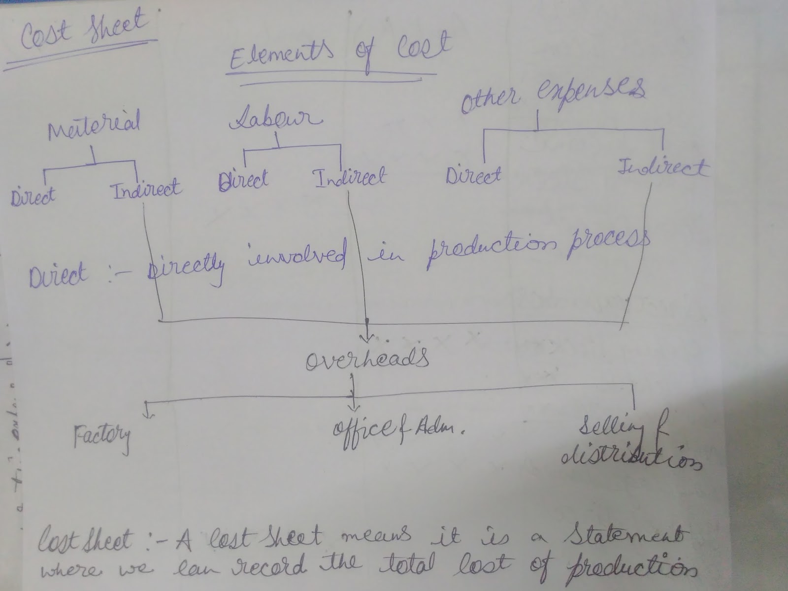
Cost Sheet
watch this video


Comments
Post a Comment